Depleted hydrocarbon fields are among the most attractive targets for geological carbon storage. A field that has trapped gas over geological time has proven its seal, its storage volume and its injectivity are constrained by decades of production data, and the pressure drop caused by production leaves room for the injected fluid. The same history makes the problem demanding to simulate. The reservoir is under-pressured, it still contains hydrocarbons that mix with the injected CO2, and the sequence of field operations (production, water injection, shut-in, CO2 injection) imposes successive pressure and saturation transients on a heterogeneous structure.
This example sets up such a case on a dome-shaped reservoir that contains the residual hydrocarbons of a previous production. It illustrates how to combine in a single GEOS input
a compositional model with four components (CH4, CO2, H2S and H2O) distributed in a gas phase and an aqueous phase, available with two alternative descriptions of the phase equilibrium: pre-tabulated equilibrium constants (K-values), or an equation of state (Peng-Robinson for the gas and Søreide-Whitson for the brine);
an initialization by capillary-gravity equilibrium around a prescribed gas-water contact in a heterogeneous structure;
three rock types, the top one being an inactive seal that is part of the mesh but not of the flow problem;
a multi-stage well schedule driven by time tables: production, water injection, shut-in and injection of a CO2-CH4 mixture, with rate targets and pressure limits on every well.
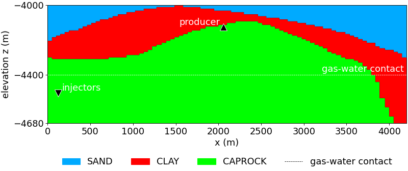
The reservoir is a dome. A sand body of good quality forms the base and the core of the structure, a clay layer of poorer quality covers it, and a caprock closes the top. The clay is thick on the flanks and thins out over the crest, where the sand comes close to the caprock. The figure below shows the rock types in the vertical section that contains the wells.
Fig. 1 Rock types of the dome, in the vertical x-z section that contains the wells. The dashed line is the gas-water contact, the triangles are the wells.
Operations
The model starts from in hydrodynamic equilibrium, with the gas-water contact at -4400 m. The field is then operated in four successive stages, summarized in the table below and in the first figure of the Results section.
The case is split in several XML files that are assembled with the Included mechanism, so that the physical model, the mesh and the fluid description can be exchanged independently. They are located in
Drivers that include one base file and one mesh file. Each one is a complete input
The results shown below are obtained with dome_soreide_whitson_bench.xml. The run is started in the usual way
geos -i dome_soreide_whitson_bench.xml
The sections below follow the order of the input and quote the files with the equation-of-state fluid, except where the K-value variant differs. The marked parts of the XML files are included directly in the text.
The mesh is read from a VTK image file (dome_bench.vti) with VTKMesh. The three wells are declared in the mesh with InternalWell: each one is a vertical polyline with a single perforation, and is linked by wellControlsName to the well definition of the solver section. The water injector and the gas injector are two separate wells that share the same trajectory, but operate at different times.
The injectors are at the bottom of the left flank, in the sand and below the gas-water contact. The producer is on the right flank, above the contact. With this arrangement the injected fluid has to travel up the structure to reach the gas that remains from the depletion.
There are 3 reservoir regions defined by 3 CellElementRegion tags in the input file. The rock is a compressible porous medium (PressurePorosity) with a constant permeability. The values given in the model are default values: the porosity and the permeability of every region are overwritten cell by cell by the FieldSpecification tags of dome_properties.xml, which scale the reference porosity and the three permeability components of each rock type:
The sand is about ten times more permeable than the clay, and in both rocks the vertical permeability is ten times smaller than the horizontal one, which makes the layering a strong control of the vertical migration of the gas.
The fluid is a mixture of four components: CH4, CO2, H2S and H2O. It is distributed in two phases, a gas phase and a water phase, by a two-phase flash. The brine density and viscosity follow the correlations of Phillips et al., with a salinity of 2.3. The pure-component data (molar mass, critical properties and acentric factor) and the binary interaction coefficients, non-zero only for the pairs that involve water, are common to the two models.
Two fluid descriptions are provided. They differ only by the way the phase equilibrium is computed, and the rest of the input is identical.
Stability analysis and flash with Peng-Robinson (gas) and Søreide-Whitson (water): the equilibrium depends on the composition
Flash with K-values read from tables of pressure and temperature: the equilibrium does not depend on the composition
Specific input
pressureCoordinates, temperatureCoordinates and the tolerances of the stability and flash algorithms
kValueTables, one table per component
Equation-of-state model
The equationsOfState attribute lists one equation of state per phase, in the order of phaseNames. The gas phase uses the Peng-Robinson (PR) cubic equation of state. The aqueous phase uses the Søreide-Whitson variant of PR, which modifies the attractive term for water and uses salinity-dependent interaction parameters, so that the solubility of the gases in the brine and the vaporization of water into the gas are represented. This matters here, since the CO2 dissolves into the brine around the plume.
The fluid properties are evaluated on a pressure-temperature grid, defined by pressureCoordinates (13 values, from 1 bar to 600 bar) and temperatureCoordinates (5 values, from 283.15 K to 354.15 K). The grid must bracket all the states visited during the simulation. Here it covers the reservoir temperature (344.15 K), the surface conditions used to convert the well rates (101325 Pa and 288.71 K) and the whole range of the well pressure limits (1 to 50 MPa).
K-value model
In the K-value variant, the fluid block is replaced by CompositionalTwoPhaseKValueFluidPhillipsBrine. The component data and the equation-of-state names are kept, but the pressure and temperature grid and the tolerances are replaced by kValueTables, which gives, for each component, the name of a table that returns the equilibrium constant as a function of pressure and temperature:
A K-value flash is simpler than a flash based on an equation of state. Its drawback is that the do not depend on the composition. It is a good choice when the compositions stay in a range for which the tables are representative, and the comparison of the two models on the same case is one of the purposes of this example.
Relative permeability and capillary pressure
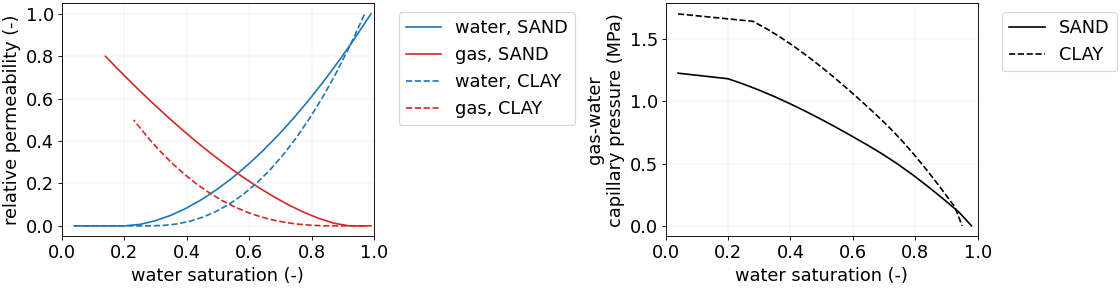
The relative permeabilities and the gas-water capillary pressures are tables of the water saturation (or of the gas saturation for the gas relative permeability), with one set per rock type. The clay uses a J-function (JFunctionCapillaryPressure), which scales a single dimensionless curve with the permeability and the porosity of each cell and with the surface tension, so that the capillary pressure adapts to the local rock quality.
<TableRelativePermeabilityname="RELPERM.SAND"phaseNames="{ gas, water }"wettingNonWettingRelPermTableNames="{ KRW.SAND, KRG.SAND }"/><TableRelativePermeabilityname="RELPERM.CLAY"phaseNames="{ gas, water }"wettingNonWettingRelPermTableNames="{ KRW.CLAY, KRG.CLAY }"/>
<TableCapillaryPressurename="CAPPRES.SAND"phaseNames="{ gas, water }"wettingNonWettingCapPressureTableName="PCGW.SAND"/><JFunctionCapillaryPressurename="CAPPRES.CLAY"phaseNames="{ gas, water }"wettingNonWettingJFunctionTableName="PCGW.CLAY"wettingNonWettingSurfaceTension="13.86955e-3"permeabilityDirection="X"/>
The curves are shown below. They show the end points given in the parameter table. The capillary pressure is of the order of 1 to 2 MPa at the irreducible water saturation, which is large compared with the gravity pressure difference between gas and water over tens of meters. This explains why a thick transition zone develops above the contact in the initial state, and why the gas needs a significant pressure to enter the clay.
Fig. 3 Relative permeabilities (left) and gas-water capillary pressures (right) of the sand (solid lines) and of the clay (dashed lines), as functions of the water saturation. The capillary pressure of the clay is obtained from its J-function with the surface tension of the model and with the clay porosity and horizontal permeability.
The temperature attribute fixes the temperature of the reservoir at 344.15 K: the energy balance is not solved. useMass="0" selects a molar formulation, so that the compositions and the injection streams are expressed as mole fractions. targetPhaseVolFractionChangeInTimeStep is relaxed to 1.0, so that the time step is selected essentially from the convergence of the Newton method.
The reservoir and the wells are solved together, in a fully implicit way, by CompositionalMultiphaseReservoir, which also holds the nonlinear and linear solver parameters:
The initial state is not uniform: the pressure, the composition and the phase saturations are set by a HydrostaticEquilibrium tag, which computes the capillary-gravity equilibrium of the whole structure from a datum and from a gas-water contact:
Datum. The pressure is 27 MPa at the elevation -4453.75 m, which is below the contact. This value is far below the pressure of about 45 MPa that a column of brine in hydrostatic equilibrium would give at this depth, as expected in a depleted field.
Contact.phaseContacts places the gas-water contact at -4400 m. The vertical pressure of each phase is integrated from the datum with the densities of the fluid, and the saturation in each cell results from the capillary pressure at its elevation above the contact. The initial gas saturation therefore increases progressively from the contact up to the crest, with a transition zone whose thickness is controlled by the capillary pressure curves of each rock type. This is why sand and clay, which have different curves, do not have the same saturation at the same elevation.
Composition. The overall composition is given as a function of elevation by one table per component, linearly interpolated between -5000 m and -4000 m. The lower part of the column is water-rich and the upper part is gas-rich, with a methane fraction that increases with elevation and a small amount of H2S. These tables represent the hydrocarbons that remain after the production.
Temperature. A constant table, equal to the temperature of the flow solver.
For instance, the tables give at the contact (-4400 m) the overall mole fractions 0.52 for CH4, 0.03 for H2S and 0.45 for H2O, with no CO2. The number of increments in the table of hydrostatic pressure is controlled by elevationIncrementInHydrostaticPressureTable, here 1 m.
Boundary conditions
No boundary condition is imposed. All the outer boundaries of the domain are closed (no-flow), so that the reservoir is a closed system in which the fluid can only enter or leave through the wells. The pressure changes are therefore driven by the compressibility of the fluids and of the rock.
Well controls
The three wells are defined in the WellManager. Each well has a main control (control), a table that gives the target rate as a function of time, and a limit on the bottom-hole pressure (BHP) that protects the well and the formation. In all of them, useSurfaceConditions="1" means that the rates are volumetric rates at 101325 Pa and 288.71 K.
The water injector injects pure water, the gas injector injects a mixture of 85 % CO2 and 15 % CH4 while the producer is controlled by the volumetric rate of the gas phase, with a lower limit on its BHP.
control="totalVolRate" with InjectionVolumeRateConstraint, injectionStream = {0, 0, 0, 1}
Injection of water at the target rate of the table WATER.INJECTOR.RATE, at the reservoir temperature. The BHP must remain below 50 MPa
Gas injector
control="totalVolRate" with InjectionVolumeRateConstraint, injectionStream = {0.15, 0.85, 0, 0}
Injection of the CO2-CH4 mixture at the target rate of the table GAS.INJECTOR.RATE, at the reservoir temperature. The BHP must remain below 50 MPa
Producer
control="phaseVolRate" for the gas phase with ProductionPhaseVolumeRateConstraint
Production at the target gas rate of the table PRODUCER.RATE. The BHP must remain above 1 MPa
The BHP constraints are safeguards. When the reservoir cannot deliver or accept the target rate within the pressure limit of the well, the rate cannot be honoured, and the pressure limit becomes the active constraint. The pressure at the well cells shown in the Results section is a useful indicator of the proximity to these limits.
Schedule
The target rates are given by three tables of the time (in seconds), which are piecewise constant (interpolation="lower"): the value at a given time is the value of the last coordinate that is not greater than this time. The first coordinate of each table, -31557600 s (one year before the start), only defines the value of the rate before the first event, which is zero.
The coordinates are multiples of one year (31557600 s). Reading the tables in years gives the schedule of the first table of this page:
the producer table, {-1,0,5,8} years with the values {0,15,15,0}, gives a production of 15 m3/s between 0 and 8 years.
the water injector table, {-1,5,8,100} years with the values {0,0.2,0,0}, gives an injection of 0.2 m3/s between 5 and 8 years;
the gas injector table, {-1,13,18} years with the values {0,20,0}, gives an injection of 20 m3/s between 13 and 18 years.
Since the producer remains open during the water flooding, the water injection is accompanied by production, and the period between 8 and 13 years, during which all the wells are closed, separates the water flooding from the gas injection.
The simulation covers 20 years. The maxTime of the events is slightly larger than 20 years (632016000 s), so that the output at 20 years is reached. The events are of three kinds.
Solver applications. The coupled solver is applied by three periodic events, which differ by the maximum time step (maxEventDt). The maximum time step is 100 days (8640000 s) before 5 years and after 5 years and 10 days. Between 5 years and 5 years and 10 days, it is limited to 1 day (86400 s), in order to handle the sudden start of the water injection. In all the cases, the actual time step is chosen by the solver from the convergence of the Newton method, and it is truncated in order to reach the output times.
Outputs. The VTK output is written every half year (15778800 s), and targetExactTimestep="1" forces the time steps to end exactly at the output times. Restart files are written every 50 cycles.
Statistics. The CompositionalMultiphaseStatistics task is executed every year (31557600 s). With computeRegionStatistics="1" and writeCSV="1", it writes the average pressure and the mass of every phase and component in each region. These files give the mass balance of the injected CO2, which is not available from the maps of the Results section.
The output and the statistics tasks are defined in the following blocks:
The VTK output of GEOS is a .pvd index file that points to one .vtm file per output time, each one being split in one .vtu file per region and per MPI rank. A couple of scripts are included for post-processing this data into and hdf5 format that can then be used to generate the images in this documentation. The scripts are:
dome_vtk_to_hdf5.py converts the whole VTK output into one HDF5 file, independent of the number of MPI ranks. It reads the .pvd file, merges the ranks of each region, orders the cells in the same way at every time, and stores the relevant datasets.
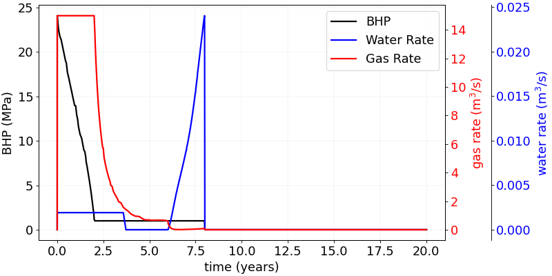
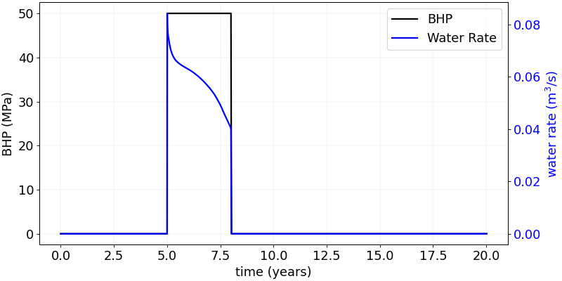
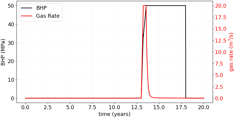
The wells do not follow the target rates of the schedule for most of the simulation. The three figures below show, for each well, the bottom-hole pressure (BHP, black, left axis) and the surface rates actually obtained (colored, right axes). When the reservoir cannot deliver or accept the target rate within the BHP limit of a well, the limit becomes the active constraint and the rate is a result of the simulation, not an input.
Producer. The producer starts at the target gas rate of 15 m3/s, with a BHP that falls from about 24 MPa. The BHP reaches the lower limit of 1 MPa after about two years, and stays there until the well is closed at 8 years. From that moment the well is controlled by the pressure limit, and the gas rate decays progressively (about 1 m3/s after five years, and close to zero after six years). The gas produced over the eight years is therefore only a fraction (roughly a third) of what the target would give. A small water rate is produced during the first 3.6 years. It is followed by a period without water, and then by a sharp increase of the water rate from about 6 years until the closure, while the gas rate is already negligible. This is consistent with the arrival of the injected water at the producer.
Fig. 5 Producer: bottom-hole pressure (black), gas rate (red) and water rate (blue). The gas rate follows the target of 15 m3/s until the BHP reaches its lower limit of 1 MPa, after about two years.
Water injector. The injector is limited by its upper BHP limit of 50 MPa from the first day of injection. The water rate peaks at about 0.085 m3/s, which is less than half of the target of 0.2 m3/s, and decreases to about 0.04 m3/s at 8 years. The injectivity is therefore low, and decreases as the pressure builds up in the closed reservoir. Only a fraction of the target volume of water is injected (well under half).
Fig. 7 Water injector: bottom-hole pressure (black) and water rate (blue). The BHP is at its upper limit of 50 MPa during the whole injection, and the rate stays below the target of 0.2 m3/s.
Gas injector. The gas injector follows the target of 20 m3/s for about half a year only. The BHP rises quickly to the upper limit of 50 MPa, and the well is then controlled by the pressure. The rate falls within one to two years to a value close to zero, and the BHP stays at 50 MPa until the end of the injection at 18 years. Almost all the CO2-CH4 mixture is injected during the first year, and the volume injected is only a small fraction of the target (roughly 10 to 15 %). The last three years of the injection period inject very little.
Fig. 9 Gas injector: bottom-hole pressure (black) and gas rate (red). The target of 20 m3/s is held for about half a year, after which the BHP reaches its upper limit of 50 MPa and the rate decays to nearly zero.
These histories show that the response of the field is controlled by the pressure limits, and that the capacity of the closed reservoir to accept fluid is the limiting factor. The producer exhausts the pressure available for production within two years. The injectors reach their pressure limit almost immediately, because the volume of the reservoir is limited and no fluid can leave it, so every volume injected increases the pressure. The stages of the schedule remain the periods during which the wells are open, but the volumes of fluid produced and injected are smaller than the targets of the input suggest.
Pressure
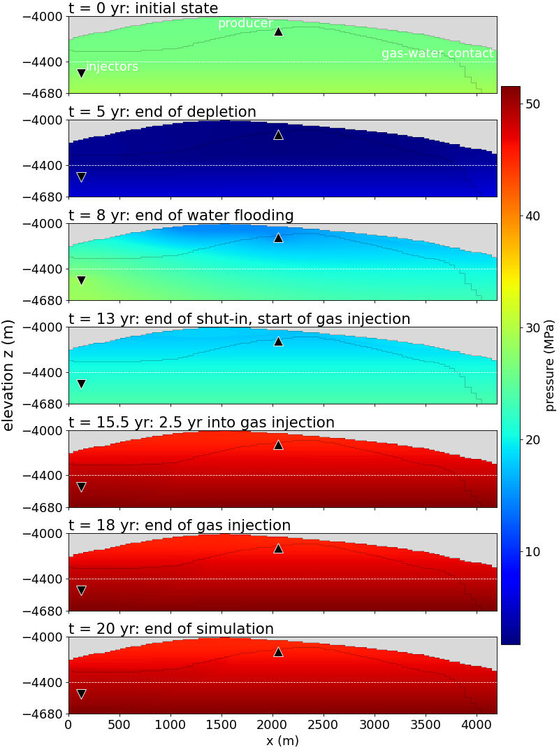
The pressure maps give the absolute pressure at the key times. The initial map is a hydrostatic distribution: the pressure increases with depth, with a gradient that changes at the gas-water contact because the gas is lighter than the water. In absolute values, the largest part of the color range is due to this vertical gradient, and the changes caused by the operations are only a fraction of it.
Fig. 11 Pressure (MPa) at the key times. The pressure increases with depth, and the gradient changes at the gas-water contact (dashed line).
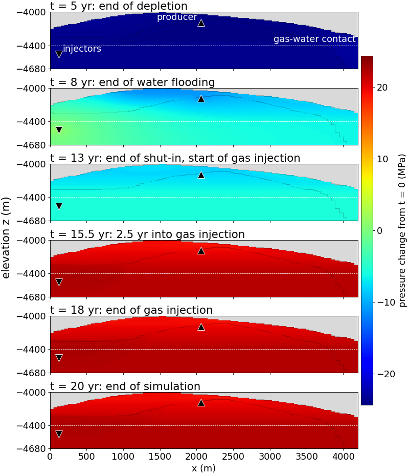
The second figure removes the hydrostatic distribution and shows the change of pressure with respect to the initial state. It is the most direct picture of the effect of the operations: blue (decrease) is created by the production, and red (increase) is created by the injections.
Fig. 13 Change of pressure with respect to the initial state (MPa) at the key times. Blue is a decrease and red an increase of pressure, on a color scale that is symmetric about zero.
Depletion (0 - 5 years). The production lowers the pressure first around the producer. The disturbance then extends toward the whole gas-filled part of the structure, and into the water leg. It travels easily in the sand and is slowed down by the clay, which has a lower permeability.
Water flooding (5 - 8 years). The pressure rises around the injector, at the bottom of the left flank. As the producer is still open, a pressure gradient develops between the two wells, and the reservoir is on average repressurized less than the injector region.
Shut-in (8 - 13 years). The pressure field becomes smoother, as the high and low pressure regions equilibrate. The map at 13 years is the starting point of the gas injection.
Gas injection (13 - 18 years). The pressure rises around the injector, and the average pressure of the reservoir increases with the injected volume. The pressure build-up at the well is the quantity to compare with the limit of the BHP.
Post-injection (18 - 20 years). The overpressure of the injector relaxes, while the plume continues to move.
Gas saturation
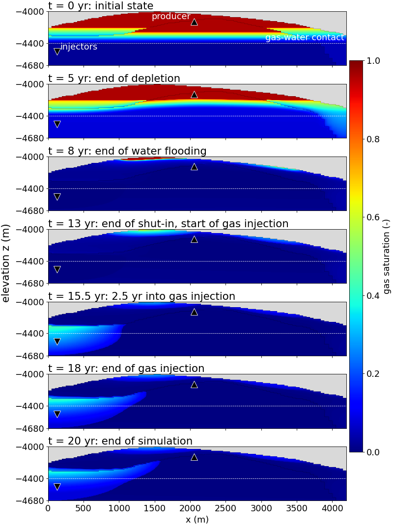
The gas saturation shows where the gas is, and its evolution is the key to understanding the other maps.
Fig. 15 Gas saturation at the key times. The gas is initially located above the gas-water contact (dashed line), with a transition zone that depends on the rock type.
At the initial time the gas occupies the upper part of the dome, above the contact. The saturation increases from the contact to the crest, with a transition zone governed by the capillary pressure curves. As the sand and the clay have different curves, the saturation changes across their interface.
During the depletion and the water flooding the injectors are below the contact, so the water that they inject mainly pushes the contact up and repressurizes the structure. The changes of gas saturation remain limited to the vicinity of the contact.
During the gas injection the gas is injected below the contact, in the water leg. As it is lighter than the water, it rises, with a plume that is formed at the injector and moves up the structure, under the clay, toward the crest, and spreads in the sand. The plume is fed during the five years of injection and its volume grows continuously.
After the end of the injection the plume keeps migrating and spreading under the effect of gravity, even if the pressure at the well relaxes. The inactive caprock closes the top of the domain. The clay, which has a lower permeability and a higher capillary pressure, slows down the vertical migration of the gas, and the gas tends to accumulate under it.
Composition: CO2 and CH4
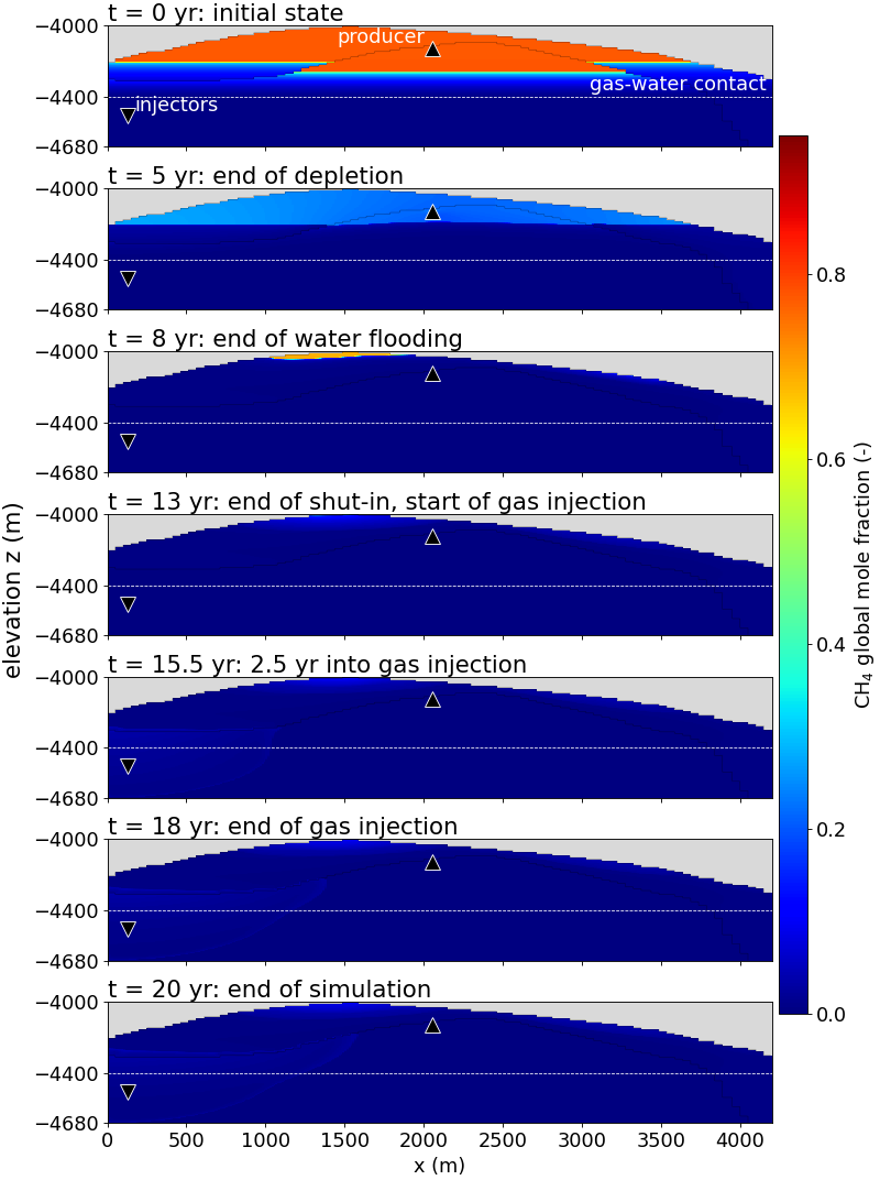
Methane. The initial map shows the native gas: an overall CH4 fraction of about 0.8 in the upper part of the dome, and essentially zero below, in the water leg. The base of the methane-rich zone lies well above the dashed line that marks the elevation given in phaseContacts.
Fig. 17 Overall mole fraction of CH4 at the key times. The native methane is produced and displaced during the first eight years, and is almost absent when the gas injection starts. The color scale is the same in all the panels.
Depletion (0 - 5 years). The overall CH4 fraction in the gas zone falls from about 0.8 to about 0.2. The production removes gas and the water takes its place, so the overall methane fraction decreases even where gas remains.
Water flooding (5 - 8 years). The methane almost completely disappears from the structure. At 8 years, only a small pocket at the very top of the dome, between about x = 1300 m and x = 1800 m, keeps an overall fraction of about 0.7. The producer cell no longer contains methane at this time. This is consistent with the producer history, where the gas rate has decayed to almost zero and the water rate increases.
Shut-in and gas injection (8 - 20 years). On a scale that goes up to 0.9 the maps are dark everywhere. The only visible traces are a few percent of methane at the top of the dome, and a very faint signature in the region of the plume, which corresponds to the 15 % of CH4 in the injected mixture.
The consequence is important for the injection stage. When the CO2 is injected, there is almost no native gas left to displace or to mix with. The plume is made of the injected mixture alone.
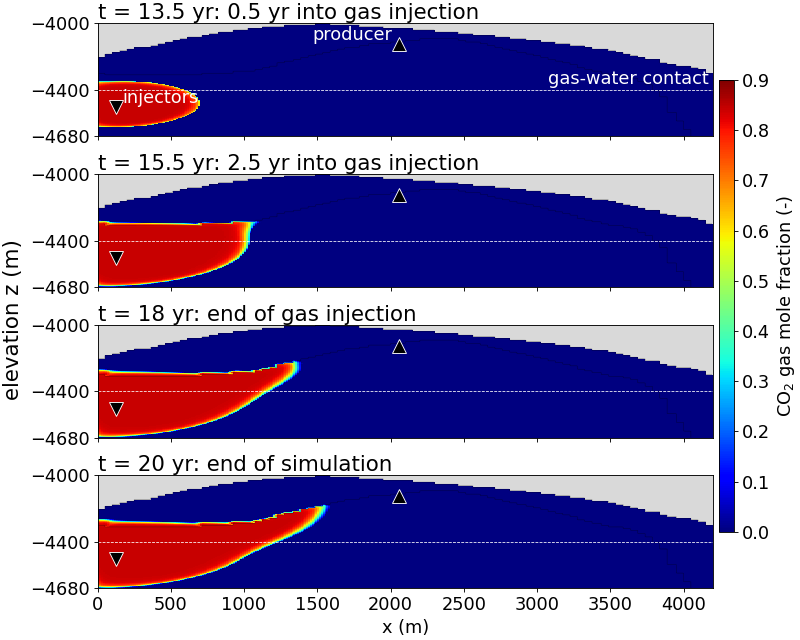
Carbon dioxide. The CO2 maps show a compact plume with a sharp boundary.
Fig. 19 Mole fraction of CO2 in the gas phase during and after the gas injection. Inside the plume the value is about 0.85, that of the injected mixture, and it is zero elsewhere. The color scale is the same in all the panels.
Inside the plume, the CO2 fraction of the gas is about 0.85 everywhere, which is the value of the injected mixture, and it is zero outside. The transition at the boundary is only a few cells thick. This agrees with the CH4 maps: the injected gas does not meet native gas on its way, so its composition is not diluted.
0.5 year after the start of the injection (13.5 years). The plume is a lens around the injectors, about 700 m wide. It extends from close to the base of the domain up to about the initial gas-water contact, above and below the depth of the injector.
2.5 years after the start (15.5 years). The plume has extended to about x = 1050 m. Its top is flat, at about -4290 m, and appears to follow the interface between sand and clay: the gas fills the sand up to the clay and is held below it. The base rises toward the front.
End of the injection (18 years). The front is at about x = 1350 m and has climbed to about -4220 m. The plume has the shape of a wedge that follows the top of the sand up the flank of the dome.
End of the simulation (20 years). The front is at about x = 1550 m and about -4180 m. Between 18 and 20 years the front advances by about 200 m, although the injector is closed at 18 years and had been injecting very little for several years before, as the history of the well shows. This late growth is driven by gravity and by the relaxation of the pressure around the well, not by the injection itself.
Near the injectors the plume fills the whole thickness of the sand, from the base of the domain to the clay. Within the 20 years of the simulation it stays on the left side of the dome. Its front remains about 500 m from the producer, and it does not reach the crest.
Conclusion
The example shows how the stages of a depleted-field storage project are driven in GEOS by time tables: production, water flooding, shut-in and CO2 injection, on a heterogeneous structure initialized by capillary-gravity equilibrium. The injection of the CO2-CH4 mixture below the contact leads to a plume that rises and spreads under the clay and the caprock, while the pressure of the field is first lowered by the production, then partially restored by the injections. The two fluid descriptions can be compared on the same case by running dome_kvalue_bench.xml instead of dome_soreide_whitson_bench.xml, converting its output, and building the pictures again.
Peng, D.-Y., and Robinson, D. B. 1976. A new two-constant equation of state. Industrial & Engineering Chemistry Fundamentals, 15(1), 59-64.
Søreide, I., and Whitson, C. H. 1992. Peng-Robinson predictions for hydrocarbons, CO2, N2, and H2S with pure water and NaCl brine. Fluid Phase Equilibria, 77, 217-240.
Phillips, S. L., Igbene, A., Fair, J. A., Ozbek, H., and Tavana, M. 1981. A technical databook for geothermal energy utilization. Lawrence Berkeley Laboratory Report LBL-12810.
 Pa-1
 m2 (316 mD),
 m2 (31.6 mD)
 m2 (31.6 mD),
 m2 (3.16 mD)
 read from tables of pressure and temperature: the equilibrium does not depend on the composition
 do not depend on the composition. It is a good choice when the compositions stay in a range for which the tables are representative, and the comparison of the two models on the same case is one of the purposes of this example.